Algorithms: Functions
What is a function and how do you define a job once and call it by name again and again? Learn parameters, RETURN, the black box and local variables — no code.
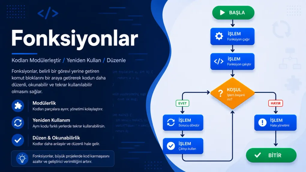
Series · Algorithms
In the previous post we learned lists and did something nice: we found the average of a list — walked it with a loop, summed it, then divided by the number of elements. Now imagine your program needs to compute that average in five different places — in a student report, a class summary, a chart. Are you going to copy-paste that loop block five times? And if you later find a bug — will you fix it in all five?
There’s a better way: give that group of steps a name, write it once, and just say its name when you need it. This named, reusable group of steps is what we call a function. That is what this post is about: defining a job once and calling it by name as many times as you like. A function sits on top of everything we’ve learned so far (variables, conditionals, loops, lists) and, for the first time, lets us break our programs into tidy pieces.
Why do we need functions?
Back to the problem from the start. Say you want to compute and print the grade average of two separate classes. Let’s deliberately write the average block from the lists post twice, so you can see the problem with your own eyes:
# Class Atotal ← 0i ← 1WHILE i ≤ length(A_grades) DO    total ← total + A_grades[i]    i ← i + 1ENDWHILEPRINT total / length(A_grades)
# Class B — the exact same steps, only the list name changedtotal ← 0i ← 1WHILE i ≤ length(B_grades) DO    total ← total + B_grades[i]    i ← i + 1ENDWHILEPRINT total / length(B_grades)
We wrote the same eight lines twice — the only difference is the list name. There are three problems. First, repetition: with a third and fourth class the code just grows and grows. Second, risk of bugs: if tomorrow you say “I computed the average wrong, I should also check for division by zero,” you have to make that fix in every copy separately; miss one and the program is right in one place and wrong in another. Third, unreadability: the code’s real intent (“take the average of two classes”) gets lost in this repeated clutter.
In everyday life we don’t fall into this trap. In a recipe you don’t rewrite “make the sauce: chop the onion, sauté it, add the paste…” from scratch every time; you describe “the sauce” once, then just say “make the sauce.” Giving a job a name and using that name — that’s the whole idea of a function.
What is a function?
A function is a name given to a group of steps. You do two separate things:
- You define it (once): You write the steps and give them a name. This does not run the steps — it just creates a recipe that sits ready.
- You call it (as often as you like): You say that name and the steps run right then. Define once, call a hundred times.
Let’s make this concrete. The simplest function just does a job, without taking or giving any information. In pseudocode we open a function with FUNCTION, write the steps indented below, and close it with ENDFUNCTION — a closing much like ENDIF from conditionals or ENDWHILE from loops:
FUNCTION greet    PRINT "Hello!"    PRINT "How are you today?"ENDFUNCTION
greet        (call it — the two lines run)greet        (call it again — they run again)
Notice: writing everything between FUNCTION greet … ENDFUNCTION prints nothing to the screen. That’s just the definition. The thing that prints “Hello!” is the greet calls below. We called it twice, it greeted twice. We wrote it once, used it as often as we wanted.
Input: giving a function information (parameters)
greet says the same thing every time. But often we want a function to behave differently depending on the situation: to greet everyone by name. For that we give the function an input. Think of a juicer: whatever fruit you put in, it gives back that fruit’s juice. A function is like that — you put a value in, it works with that value.
We give the input a placeholder name inside the definition; this is called a parameter. When calling, we put a real value in place of that placeholder; this is called an argument:
FUNCTION greet(name)    PRINT "Hello, " + name + "!"ENDFUNCTION
greet("Ada")     → Hello, Ada!greet("Can")     → Hello, Can!
The + here is the text concatenation you know from the variables post. The name in the definition is a parameter — waiting like an empty box. When you say greet("Ada"), the argument "Ada" goes into that box and the function uses “Ada” everywhere it sees name. On the next call, “Can” goes into the box. The same function does a different job with different input.
Output: getting a result from a function (RETURN)
Our functions so far did a job but gave back no result. Yet often we want a function to compute something and hand it back to us — like a calculator that gives the answer and waits. A function handing back a result is called RETURN:
FUNCTION square(n)    RETURN n × nENDFUNCTION
result ← square(5)   (square(5) returns 25; that 25 goes into result)PRINT result         → 25
The square(5) call runs, computes 5 × 5 = 25, and with RETURN hands 25 back to the caller. Notice we can put that returned 25 into a variable (result) — this is where a function’s power lies. Now square is like a tool that produces numbers; you can put its output wherever you like: PRINT square(3), area ← square(side), even square(square(2)) (the square of the square of 2 = 16).
You can picture what happens in a function call like this: the main program pauses for a moment and sends the argument to the function; the function does its job and hands the result back with RETURN; the main program takes that result and continues where it left off:
flowchart TD
    A["Main program<br/>result ← square(5)"] -->|"5 is sent in (argument)"| B["square(n) function<br/>RETURN n × n"]
    B -->|"25 comes back (RETURN)"| C["Main program continues<br/>result is now 25"]
Notice the arrow going into the function and coming back with a value — a call hands the program’s flow to the function for a moment, and RETURN brings the result back. Here we reach the point beginners confuse most often:
Input and output together: a real function
Now let’s put the pieces together and solve the problem from the start of this post. Let’s turn the average block from lists into a real function that takes an input (a list) and returns an output (the average):
FUNCTION average(list)    total ← 0    i ← 1    WHILE i ≤ length(list) DO        total ← total + list[i]        i ← i + 1    ENDWHILE    RETURN total / length(list)ENDFUNCTION
PRINT average(A_grades)      (Class A's average)PRINT average(B_grades)      (Class B's average)PRINT average([100, 90, 80]) (you can call it with a ready list too → 90)
Look how that two-copy, long block from the start of the post melted away: we wrote the average logic once, then just called it for three different lists. If tomorrow you say “let me check for division by zero,” you make the fix in one place — inside the function — and all the calls fix themselves. That’s exactly what functions promised.
Notice how everything we’ve learned in this series works together inside: a list parameter, a loop, an accumulator (total), a variable (i), and finally a RETURN. The function hides all these pieces behind a single name.
In fact, the inside of a function is an algorithm with two defined ends, just like the ones we’ve drawn in this series: it enters with parameters and exits with RETURN. If we draw the steps inside average as a flowchart, we get the familiar diagram from the loops post, now wrapped inside a function’s boundaries:
flowchart TD
    A(["average(list) is called"]) --> B["total ← 0<br/>i ← 1"]
    B --> C{"i ≤ length(list)?"}
    C -- Yes --> D["total ← total + list[i]"]
    D --> E["i ← i + 1"]
    E --> C
    C -- No --> F(["RETURN total / length(list)"])
The rounded box at the top is where the function is called (starts); the box at the bottom is where it hands back the result and exits — RETURN is the function’s version of an algorithm’s “Done” end. A function is nothing more than a named algorithm with two defined ends like this.
Think of a function as a “black box”
Now we reach the real magic of functions. When you call the average above, did you think about whether there’s a loop inside, how it sums? You don’t need to. When you write average(A_grades), all you know is: you give a list, you get back an average. The inside is a black box to you — you know what goes in and what comes out, you don’t need to know how it works inside.
flowchart LR
    A["Input (parameter)<br/>list = [90, 80, 100]"] --> B["average<br/>BLACK BOX<br/>(the inside doesn't concern us)"]
    B --> C["Output (RETURN)<br/>90"]
Whether there’s a loop inside the middle box or some other method makes no difference from the outside; you just give the input on the left and take the output on the right. This is something you do everywhere in life:
- A TV remote: you press a button, the channel changes. You don’t need to know the infrared signal, the circuits inside.
- A microwave: you put the food in, set the time, press start. You don’t deal with what happens inside.
- A tap: you turn it, water comes. You don’t think about which pipes and which pump it came through.
A function’s inside is its own: local variables
Inside the average function we used two variables, total and i. Do these names exist outside the function too? No. Variables defined inside a function live only there; they disappear when the function ends and can’t be seen from outside. These are called local variables; they’re like a function’s own private scratchpad.
Why is this a good thing? Because two different functions can use the same name without clashing at all. average has an i inside it; another function can have an i too; they’re entirely different boxes, neither overwrites the other. Each function works comfortably in its own corner, with its own variables.
A function calls a function
Functions have one more beauty: from inside one function you can call another function. You build bigger jobs by combining small pieces. For example, let’s produce both the average and a “did they pass?” result from a student’s grades; the second uses the first:
FUNCTION passed(list)    avg ← average(list)          (calling the function we defined above)    IF avg ≥ 50 THEN        RETURN true    ELSE        RETURN false    ENDIFENDFUNCTION
PRINT passed([70, 40, 55])    → true   (average is 55, passed)
passed doesn’t compute the average itself — it delegates that job to the average function that knows how, evaluates the returned result with a conditional, and returns true/false (a boolean). This is how you build big jobs from small, single-purpose pieces. Note: a function like passed that returns true/false can be seen as “a function that asks a yes/no question” — like isEven, isEmpty, isValid.
Built-in functions: don’t reinvent the wheel
As the tip above hinted, every programming language comes with pre-written functions for common jobs: printing to the screen, getting a list’s length, computing a square root, converting text to uppercase… These are called built-in functions, and collectively a library. The goal is simple: don’t reinvent the wheel. You don’t write a square-root algorithm from scratch every time; you call the ready-made function the language gives you and focus on your real work.
Real programming is largely this: combining functions — some you wrote, some ready-made — by their names, building bigger jobs layer by layer. Each function is a brick; the program is the building you make from those bricks.
Common mistakes
Try it yourself
Pen and paper are enough. For each exercise, first define the function (FUNCTION … ENDFUNCTION), then call it with a few different arguments and trace the result on paper. Don’t forget the distinction between input (parameter) and output (RETURN).
Exercise 1 — Return the larger one (easy)
Write a
larger(a, b)function that takes two numbers and returns the larger one. Then call it withlarger(3, 9)andlarger(12, 7)and print the results.
Exercise 2 — Is it even? (medium)
Write an
isEven(n)function that takes a number and returnstrueif it’s even,falseif it’s odd. Try it withisEven(4)andisEven(7).
Exercise 3 — A function that sums a list (medium)
Write a
sum(list)function that takes a number list and returns the sum of its elements. Then call it with two different lists:sum([10, 20, 30])andsum([5, 5, 5, 5]).
Exercise 4 — Report card: combine functions (mini project)
Write an
average(list)function (use the one from the post) and ahighest(list)function (returns the biggest element). Then, for a listgrades ← [65, 90, 78, 55], call both and print a report card in the form “Average: … , Highest: …”.
Summary
Related posts
Frequently asked questions
What is a function?
A function gives a name to a group of steps, making them a single unit: you define it once, then run it as many times as you want by saying its name (calling it). Like naming a step in a recipe — you say "make the sauce" instead of rewriting all the steps. It is the way to reuse the same work in different places and to break a complex program into small, named pieces.
Why do we use functions?
Three big reasons. They avoid repetition: you write the same steps once instead of copy-pasting them (if a bug turns up, you fix it in one place). They break up complexity: you split a long program into small named pieces, each doing one job. And they hide detail: to use a function you do not need to know how it works inside, only what you give it and what you get back.
What is the difference between a parameter and an argument?
A parameter is the placeholder name you use when defining the function (the "name" in FUNCTION greet(name)). An argument is the real value you put into that placeholder when calling it (the "Ada" in greet("Ada")). In short: the parameter is the "an onion" written in the recipe, the argument is the actual onion in your hand. The argument can change on every call; the parameter name stays the same.
What is the difference between RETURN and PRINT?
PRINT puts a value on the screen — a human sees it, but the program cannot do anything more with it. RETURN hands the result back to the caller, so you can put it in a variable, feed it into another operation, or pass it to another function. PRINT is for showing, RETURN is for handing back a usable result. This is the distinction beginners most often confuse.
What is a local variable (scope)?
A variable defined inside a function lives only there; it disappears when the function ends and cannot be seen from outside. This is called a local variable. It is like the function's own private scratchpad. Thanks to this, two different functions can use the same name (say i or total) without clashing; each gets its own copy.
What is the difference between defining and calling a function?
Defining writes the function's steps once and gives them a name — but it does not run the steps, it just creates a recipe that sits ready. Calling says that name and runs the steps right then. If you define a function but never call it, nothing happens; just like writing a recipe but never cooking it.
What is a built-in function?
Programming languages come with pre-written functions for common jobs — you use them without writing them. length, which gives a list's length, PRINT, which writes to the screen, and taking a square root are examples. Collections of these ready-made functions are called libraries. The goal is not to reinvent the wheel: take the basics ready-made and focus on your real work.
Why is a function compared to a "black box"?
Because to use a function you do not need to know what happens inside; you only need to know what you give it (input) and what you get back (output). Just like a TV remote or a microwave: you press a button, the job gets done, and you do not deal with the electronics inside. This idea of "hiding the inside" is called abstraction, and it is what makes large programs manageable.